II. CMB background
This post is a historical background overview of CMB science.
The CMB prediection by Ralph Alpher (George Gamow's Ph.D.) and Robert Herman in about 1948. This is a list of historical paperss from 1965 to 2018 which may provide useful background in CMB (reference BICEP's internal group!).
- 1965: The accidental discovery by Penzias and Wilson using a horn antenna at Bell laboratory
- A Measurement of Excess Antenna Temperature at 4080 Mc/s
A. A. Penzias and R. W. Wilson, ApJ 142, 419(1965). - 1981: A. Guth's initial paper of an inflation universe
- Inflationary universe: A possible solution to the horizon and flatness problems
A. Guth, Phys. Rev. D 23, 347 (1981). - 1982: Linde's initial paper on inflation, addressing some of the self-admitted problems with Guth's model
- A new inflationary universe scenario: A possible
solution of the horizon, flatness, homogeneity, isotropy,
and primordial monopole problems
A.D. Linde, Phys. Lett. B 108, 389 (1982). - 1992: First detection of temperature anisotropy in the CMB by COBE satellite. COBE also measureed the spectrum of CMB as a black body with temperature of 2.725 K.
- Structure in the COBE Differential Microwave Radiometer
First-Year Maps
G. Smoot et al., ApJL 396, L1 (1992). - 1997: Seljak and Zaldarriaga's paper initially describing the E and B decomposition of CMB polarization as a way of probing for primordial gravitational waves from the Big Bang, starting the time for CMB polarization measurement experiment.
- Signature of Gravity Waves in the Polarization of the
Microwave Background
U. Seljak and M. Zaldarriaga, Phys. Rev. Lett. 78, 2054 (1997). - 1997: Kamionksowski, Kosowsky, and Stebbins' paper also deriving the E and B basis, in a slightly different way than Seljak and Zaldarriaga, published alongside said paper
- A Probe of Primordial Gravity Waves and Vorticity
M. Kamionkowski, A. Kosowsky, A Stebbins, Phys. Rev. Lett. 78, 2058 (1997). - 2002: First detection of polarization in the CMB E modes by DASI
- Detection of polarization in the cosmic microwave background using DASI
J.M. Kovac et al., Nature 420, 772 (2002). - 2014: BICEP claim CMB B mode (tensor-to-scalar ratio) r < 0.2 detection, but later join analysis with Planck confirm there has contamination from foreground
- Detection of B-Mode Polarization at Degree Angular Scales by BICEP2
BICEP Rev. Lett. 112, 241101, 2014 - 2018: Planck Satellite's latest (2018) results on cosmological parameters
- Planck 2018 results. VI. Cosmological Parameters
Planck Collaboration et al., A&A 641, A6 (2020). - 2018: Planck Satellite's latest (2018) constraints on inflation (using BICEP/Keck's "BK15" data set)
- Planck 2018 results. X. Constraints on inflation
Planck Collaboration et al., A&A 641, A10 (2020). - 2022: The upper limit on tensor-to-scalar r < 0.032 (95% CL). using BICEP and Planck data
- Improved limits on the tensor-to-scalar ratio using BICEP and
Planck data
M. Tristram, et al., Phys. Rev. D 105, 083524 – Published 26 April 2022 - 1997: A pedagogical introduction to CMB polarization. Includes a description of how polarization is generated during recombination, a breakdown of E and B and how they relate to Q and U, etc.
- A CMB Polarization Primer
W. Hu and M. White, New Astron. 2, 323 (1997). - 2016: A nice review on the CMB polarization
in 2016, - The Quest for B Modes from Inflationary Gravitational Waves
Marc Kamionkowski and Ely D. Kovetz annual reviews
There are several nice papers to look at
There are many good books in the field,
- An Introduction to Modern Cosmology, Andrew Liddle 3rd Edition
- This is a good book for the beginner, it covers all the important aspect in Cosmology
- Introduction to Cosmology, Barbara Ryden 2nd Edition
- This books describe detail calculation of Universe models, problem and solutions to the Big Bang Universe.
- Modern Cosmology, Scott Dodelson, Fabian Schmidt 2nd Edition
- This is a good book for graduate level and researcher.
- Cosmology, Daniel Baumann
- This is resource for advanced students in theoritical physics, cosmology.
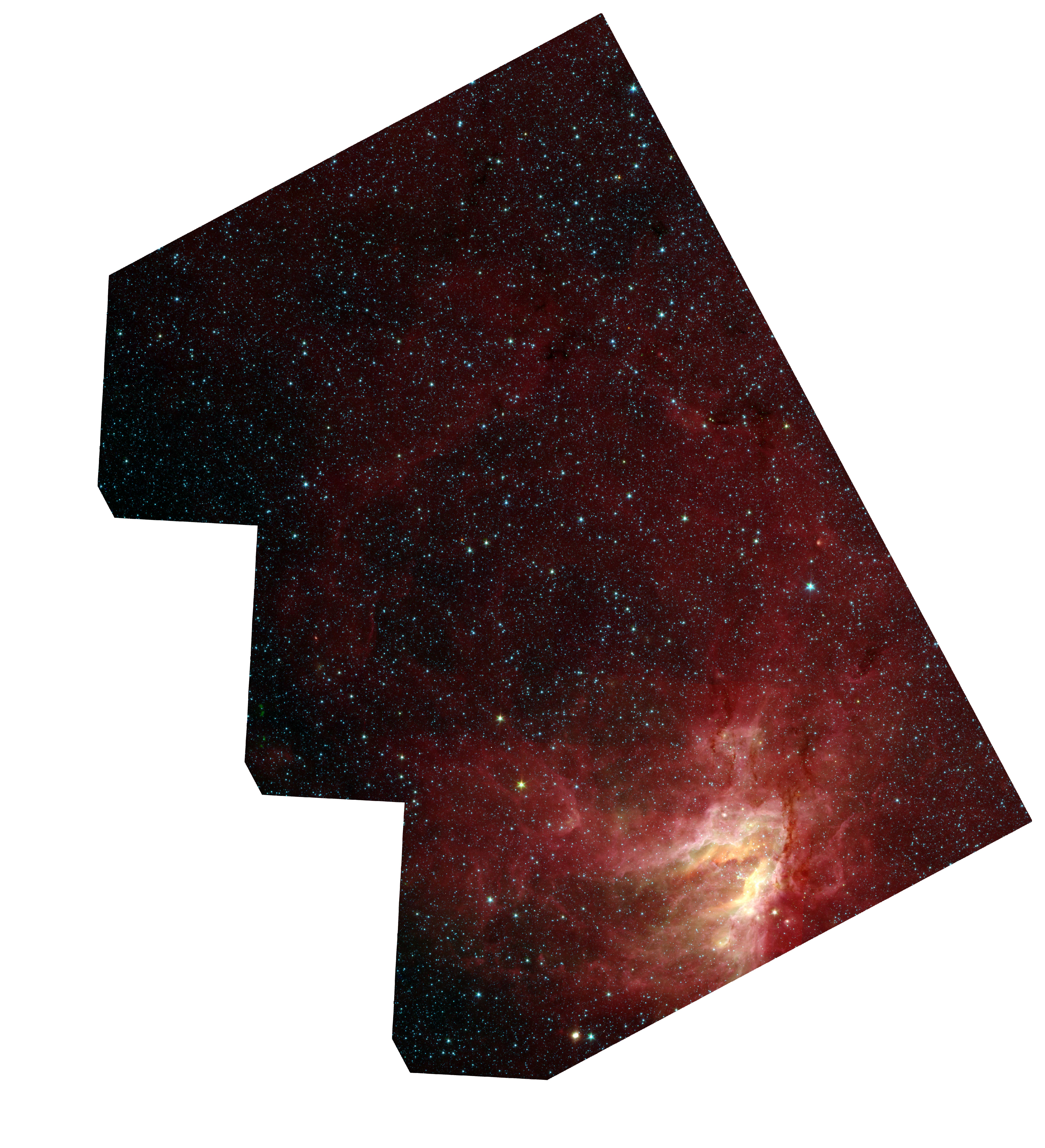
I. How to make an RGB image using aplpy package
This is an example of making a RGB image using aplpy package.
The data is archived from the Spitzer Galactic Legacy Infrared Midplane Survey Extraordinaire
(GLIMPSE).
We will choose 3 over 4 channels data to generate an RGB optical-liked image of M17 region
(Omega Nebula/Swan Nebula/Horseshoe Nebula)
...Read More